Projective Dynamics Presentation on Seminar

Projective Dynamics

: vertices

: positions

: velocities

: the sum of external forces

: the sum of internal forces

: position dependent internal forces

: scalar potential energy function

State at :

Implicit Euler Solver

step size: : :

plug (2) into (1)

Let (explicit), we get

It is equivalent to the minimization problem

(reason: the derivative of Eq.(4) is Eq.(3))

Interpretation

• : Inertia & external force term (momentum potential)
• : Internal energy term. (e.g. Simple FEM energy: )

So, the minimization is trying to find the balance between the inertia & external forces term and the internal energy term.

Imagining a moving jellow, for every particle on it, it has to find a compromise between the momentum and self deformation. (deforming and moving at same time)

Elastic Potentials

• defines a constraint manifold of all possible undeformed configurations, while measures how far the deformed configuration is from this manifold.

Author decoupled these 2 concepts through a projection auxiliary variable :

potential functions defines as represents the distance between and

, which from geometric point of view, only equals 0 when is on the constraint manifold.

So minimizing over is finding the projection of on the constraint manifold.

More generally, can be defined as where and is constant matrices and is a nonnegative weight.

Projective Implicit Euler Solver

Eq.(4) became the minimization of over and the auxiliary variables . is selection matrix that selects the vertices involved in the th constraint.

Local Solve

fix , minimize Eq.(5) over

and is a stack of all particles per constraint (for two connected spring constraints, should be the endpoints of each spring) first term is irrelevant

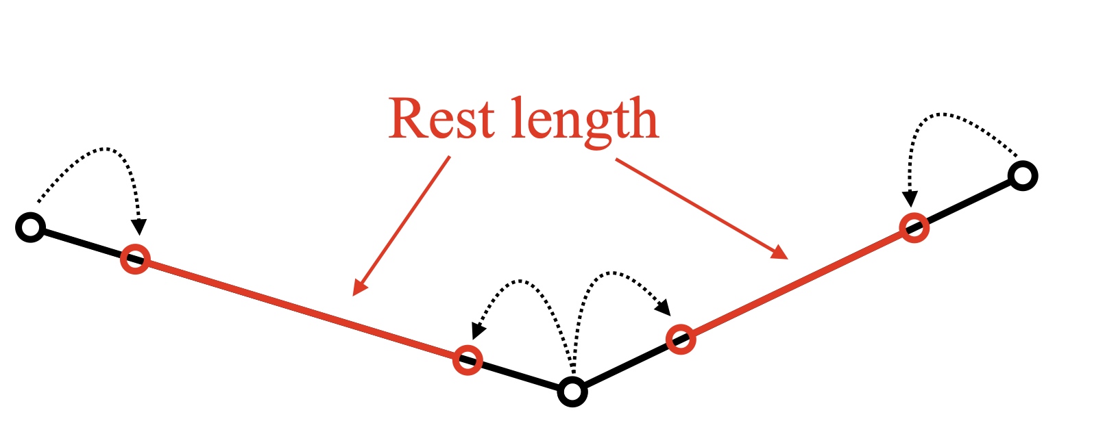
Intuitively, the local step means projecting each constraint to its rest state.

Global Solve

fix , minimize Eq.(5)

when fixing , should be 0 which means should be on the manifold.

Expand the second term, we get

taking the derivative of Eq.(6) over (indicator function will be discarded)

with simple transformation

Let be . is constant as long as the constraint are not changing.

through sparse Cholesky decomposition, .

and the right hand side will keep changing due to . And we can solve like this

Intuitive explanation

Local Step

taking mass-spring system as example. Imagining 2 extended springs connected together. what local solve does is project each spring into their rest length. After that, two springs will be detached and connected point(particle) will be duplicated.

Local Solve

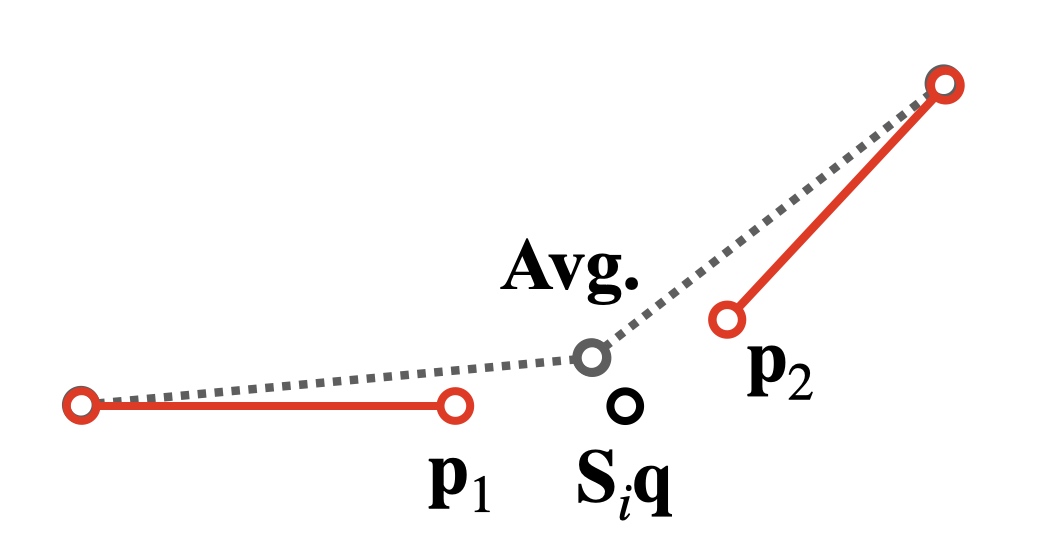
Global Step & Choice of A and B

The global solve will bring these two springs connected again. Recall that there are two constant metrics , which actually control how we measure the quadratic distance.

For simplest case: , after each spring has been projected on its rest length, inertia & external forces term of Eq.(5) and will be both equal to 0. Only internal energy term is left for minimization. So we can compute the gradient of potential energy and set it to zero.

the result is , which means simply doing averaging.

Global Solve

This leads to poor convergence rate. As shown below, if i pull the corner of this mass-spring cloth, the change propagates to the end will be very slow if are identity and will cause stretchy artifacts.

Global Solve

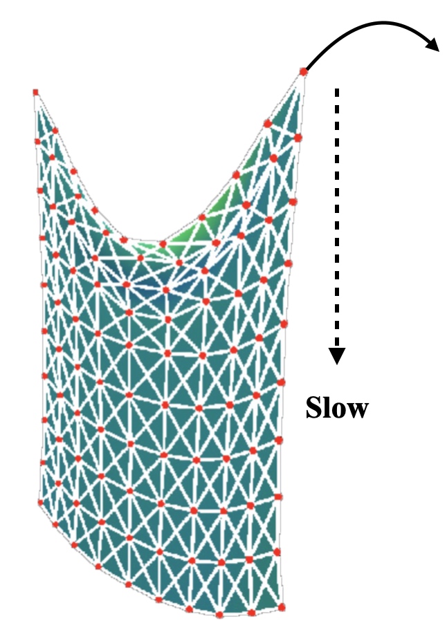
better choice

where is a p by p identity, is a p by p matrix of ones, p is the number of particles involved in current constraint.

For the connected two springs system, it will became By doing this, will subtract the mean of current state and the projection , so the global step can translate the constraints. (translation invariant)